By
Machine learning has achieved many successes in a wide range of application areas, but more often than not, these strongly rely on choosing the correct values for many hyperparameters (see e.g. Snoek et al., 2012). For example, we all know of the awesome results deep learning can achieve, but when we set its learning rates wrongly it might end in total disaster. And there are a lot of other hyperparameters, e.g. determining architecture and regularization, which you really need to set well to get strong performance. A common solution these days is to use random search, but that is very inefficient. This post presents BOHB, a new and versatile tool for hyperparameter optimization which comes with substantial speedups through the combination of Hyperband with Bayesian optimization. The following figure shows an exemplary result: BOHB starts to make progress much faster than vanilla Bayesian optimization and random search and finds far better solutions than Hyperband and random search.
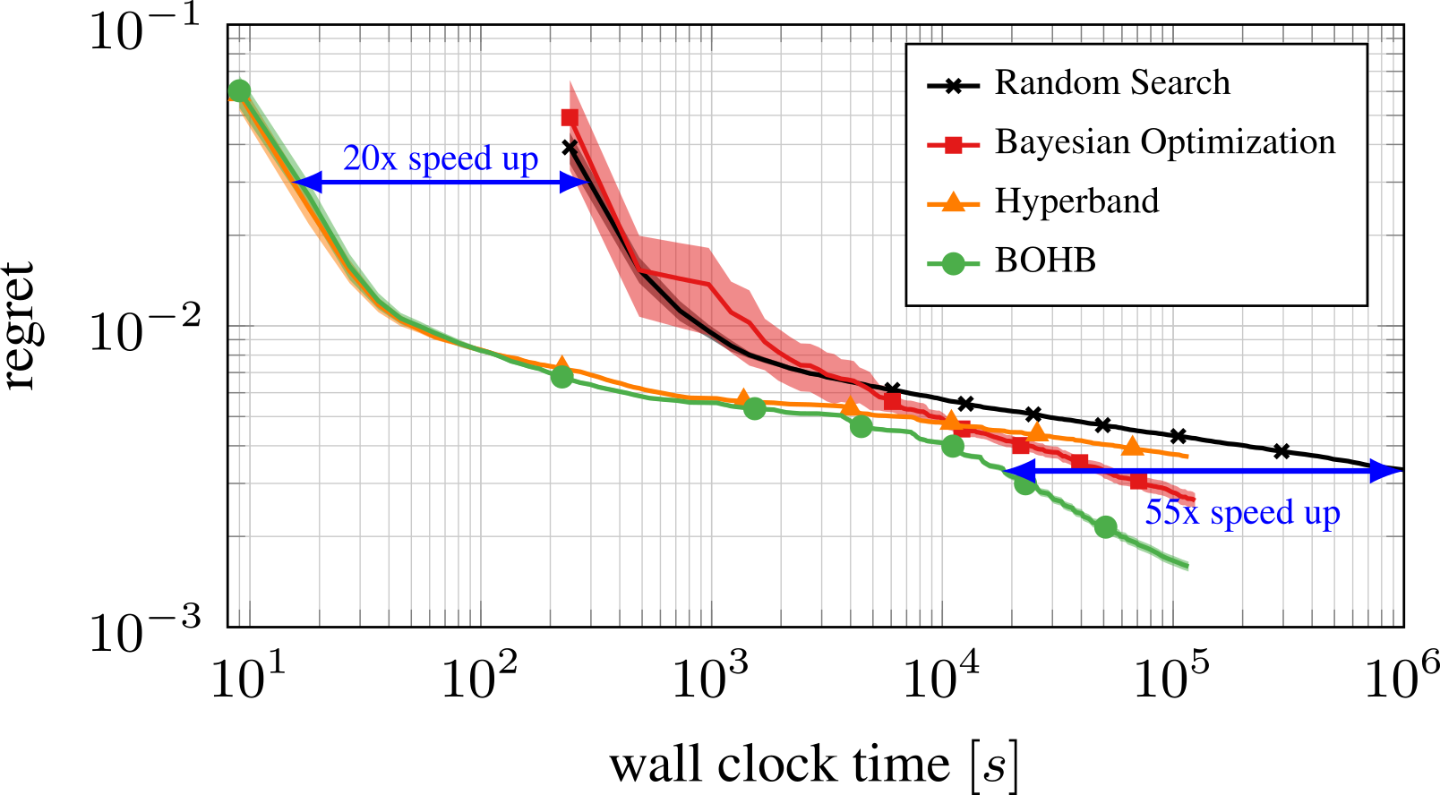
Example results of applying BOHB (freely available under https://github.com/automl/HpBandSter) to optimize six hyperparameters of a neural network. The curves show the immediate regret of the best configuration found by the methods as a function of time. BOHB combines the best of BO and Hyperband: it yields good performance (20x) faster than BO in the beginning, and converges much faster than Hyperband in the end.
BOHB is freely available under https://github.com/automl/HpBandSter.
Desiderata for a practical solution to the hyperparameter optimization problem
The setting above leaves us with a variety of desiderata for a practical solution to the hyperparameter optimization (HPO) problem in deep learning that BOHB was designed to tackle:
- Strong Anytime Performance: Most practitioners and researchers only have enough resources available to fully evaluate a handful of models (e.g. large neural networks). HPO methods should be able to yield good configurations in such small budgets.
- Strong Final Performance: After the development phase, for use in practice, what matters most is the performance of the best configuration that a HPO method can find. Methods based on random search lack guidance and therefore struggle to find the best configurations in large spaces.
- Effective Use of Parallel Resources: Practical HPO methods need to be able to use the ever-more available parallel resources effectively.
- Scalability: Practical HPO methods also need to be able to handle problems ranging from just a few hyperparameters to many dozens.
- Robustness & Flexibility: HPO challenges vary across different fields of machine learning. For example, deep reinforcement learning systems are known to be very, very noisy. Different optimization problems also come with different types of hyperparameters, including Boolean choices, discrete parameters, ordinals or continuous choices.
- Simplicity: Simple methods have fewer components, should be less prone to failure, can easily be verified and are easy to (re-)implement in different and new frameworks.
- Computational efficiency: Parallel HPO methods might be able to carry quite a lot of function evaluations. A model that guides the hyperparameter optimization has to be able to handle the resulting amount of data efficiently.
To fulfill all of these desiderata BOHB combines Bayesian optimization with Hyperband.
Bayesian Optimization and Hyperband
The validation performance of machine learning algorithms can be modelled as a function of their hyperparameters. The HPO problem is then defined as finding the hyperparameter setting that minimizes this objective function. Bayesian optimization (BO; Shahriari et al., 2016) and Hyperband (HB; Li et al., 2016) are two methods for tackling this problem.
Bayesian Optimization
BO uses a probabilistic model to model the objective function based on the set of already observed data points (Shahriari et al., 2016). BO uses an acquisition function based on the current model to identify promising new configurations. The standard BO process then iterates over the following three steps:
- Select the point that maximizes the acquisition function
- Evaluate the objective function at this point
- Add the new observation to the data and refit the model
The trade-off between exploration and exploitation can be controlled via the acquisition function. As BO needs time to build a good model that will lead to better performing configurations, in its vanilla version, BO behaves similarly to Random Search in the beginning. With increasing budgets, however, the model gathers more and more information about the search space, leading to great advantages over Random Search. An example of this is shown below.
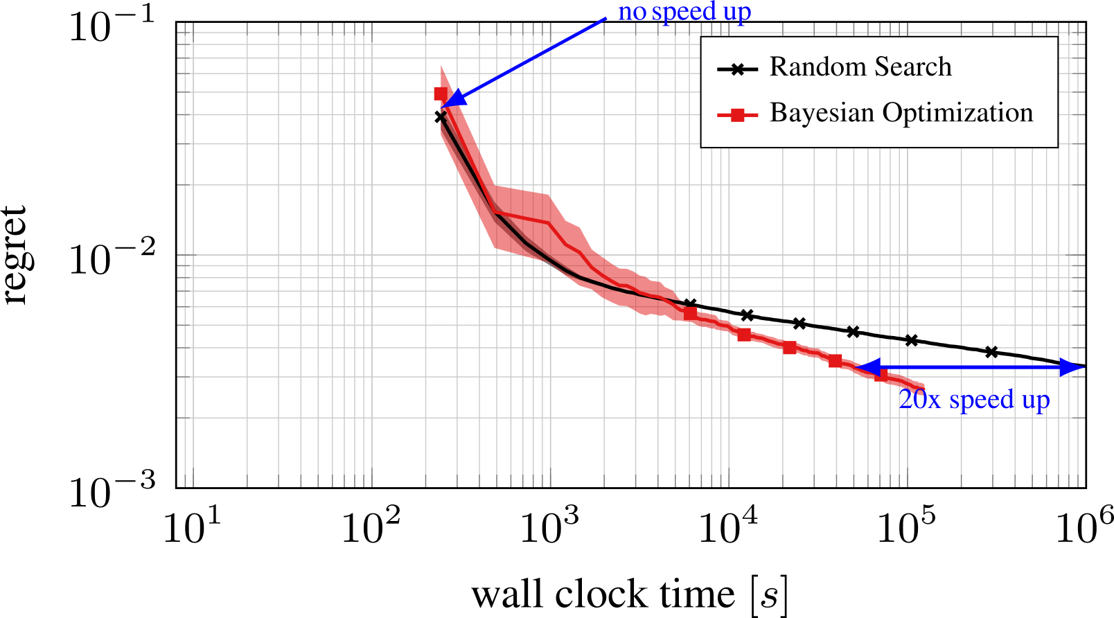
BO substantially outperforms Random Search for larger budgets.
For this plot we used a vanilla version of BO. There are multi-fidelity variants of BO (such as Fabolas; Klein et al., 2017), which improve over vanilla BO. However, due to being based on GPs they don’t fulfill some of the given desiderata (scalability, robustness, flexibility, etc). Later we showcase how such multi-fidelity variants compare to Random search and BOHB when optimizing an SVM on the MNIST dataset.
Hyperband
Hyperband (HB; Li et al., 2016) is an HPO strategy that makes use of cheap-to-evaluate approximations of the objective function on smaller budgets. HB repeatedly calls SuccessiveHalving (SH; Jamieson et al., 2016) to identify the best out of n randomly-sampled configurations. In a nutshell, SH evaluates these n configurations with a small budget, keeps the best half and doubles their budget; see the figure below for a visualization.
SuccessiveHalving starts by randomly sampling n configurations. In each iteration it drops the worst half and doubles the budget for the rest until it reaches the maximum budget. Each line corresponds to a configuration.
Hyperband balances very aggressive evaluations with many configurations on the smallest budget and very conservative runs on the full budget. This helps it guard against having trusted cheap budgets too much.
In practice HB performs very well for small to medium budgets and typically outperforms random search and vanilla BO quite easily in that setting. However, its convergence is limited by its reliance on randomly-drawn configurations: with larger budgets its advantage over random search diminishes. An example of this is given in the plot below.
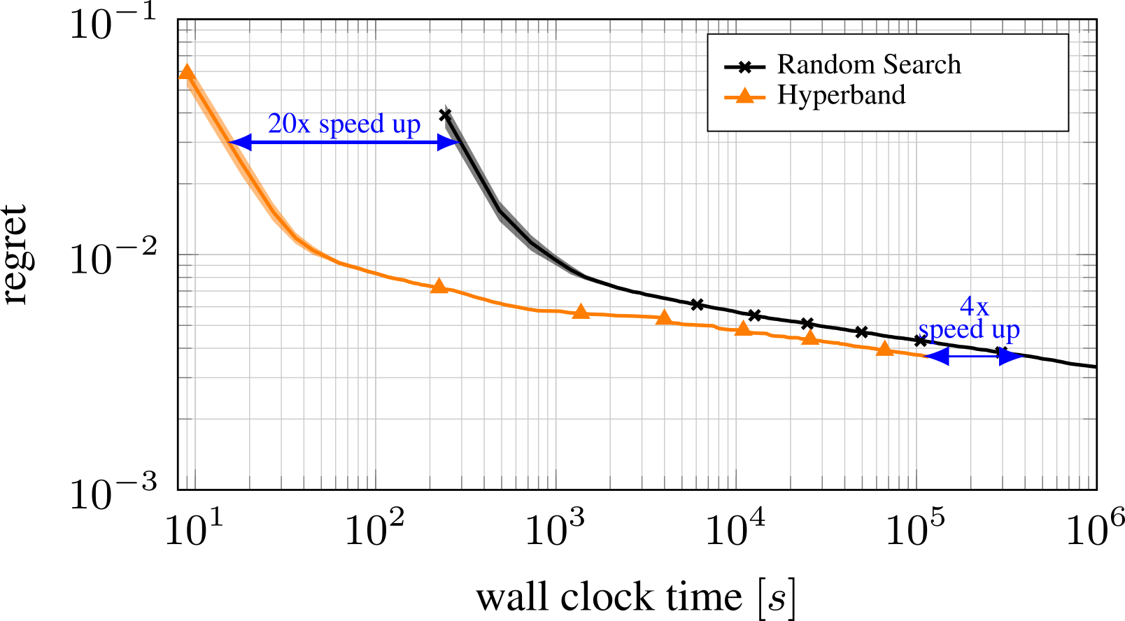
With increasing budget, Hyperband’s advantage over Random search diminishes.
Since BO behaves similarly to Random Search in the beginning, Hyperband exhibits the same advantage over BO for small to medium budgets. For bigger budgets, BO’s model typically guides the search to better-performing regions and BO outperforms Hyperband.
Robust and Efficient Hyperparameter Optimization at Scale
Illustration of typical results obtained exemplary for optimizing six hyperparameters of a neural network. The curves give the immediate regret of the best configuration found by 4 methods as a function of time.
BOHB combines Bayesian optimization (BO) and Hyperband (HB) to combine both advantages into one, where the Bayesian optimization part is handled by a variant of the Tree Parzen Estimator (TPE; Bergstra et al., 2011) with a product kernel (which is quite different from a product of univariate distributions). BOHB relies on HB to determine how many configurations to evaluate with which budget, but it replaces the random selection of configurations at the beginning of each HB iteration by a model-based search, where the model is trained on the configurations that were evaluated so far.
BOHB’s strong anytime performance (desideratum 1) stems from its use of Hyperband. Quickly evaluating lots of configurations on small budgets allows BOHB to quickly find some configurations that are promising. The strong final performance (desideratum 2) stems from BOHB’s BO part as the guided search in the end is able to refine the selected configurations.
The plot at the top of the section shows that BOHB behaves like Hyperband in the beginning and later profits from the constructed BO model. In the beginning, both BOHB and Hyperband show a 20x speedup over Random Search and standard BO. With increasing budgets, Hyperband’s improvement over Random Search diminishes but BOHB still continues to improve, with a speedup of 55x over Random Search.
BOHB also efficiently and effectively takes advantage of parallel resources (desideratum 3). In each iteration BOHB is evaluating multiple configurations, which can be independently run on multiple workers. This can significantly speed up the optimization process. An example of BOHB’s performance for different numbers of parallel workers is given below.
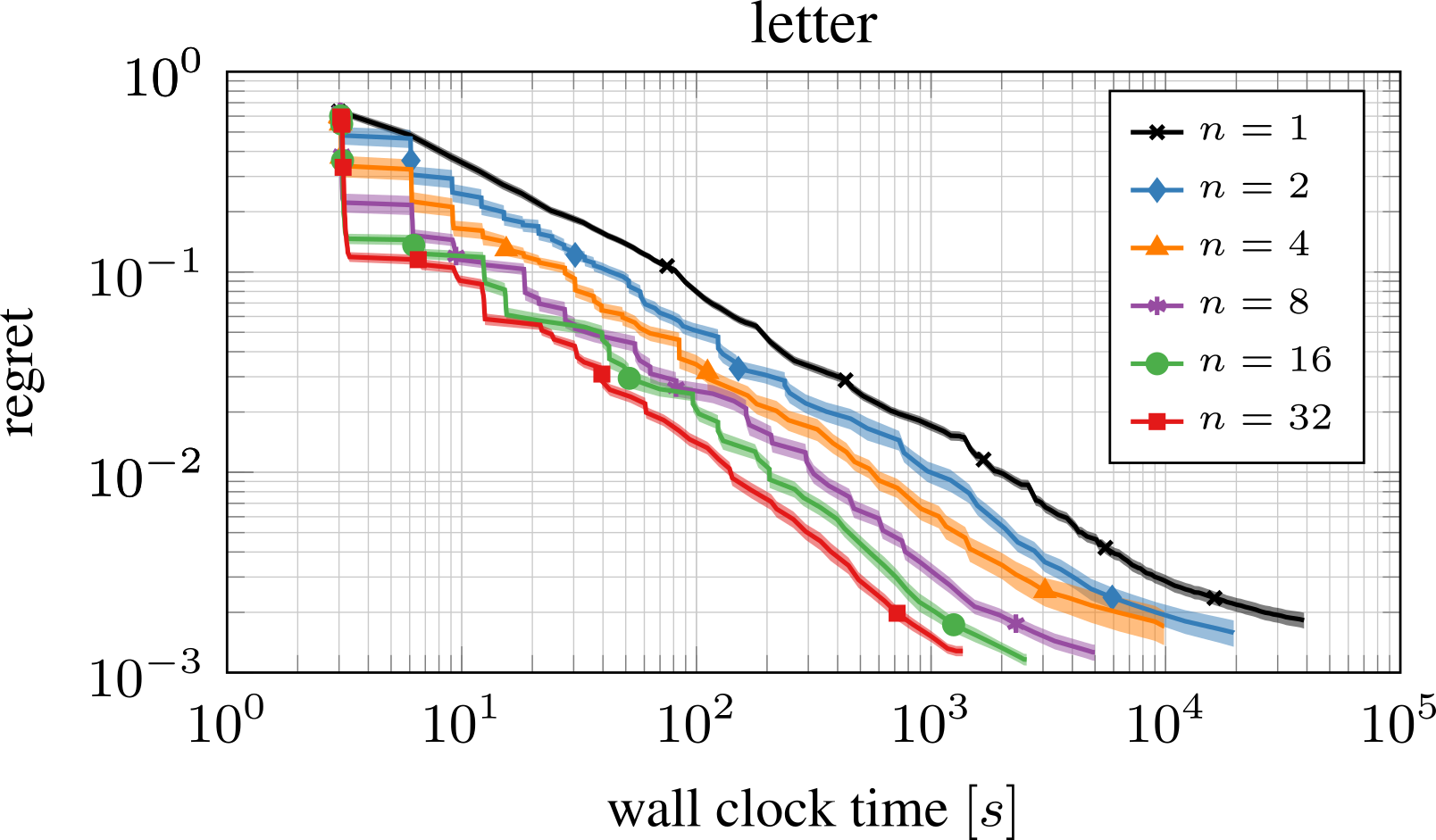
Performance of BOHB with different number of parallel workers for 128 iterations on the surrogate letter benchmark. The speedups are close to linear.
Applications
BOHB has been evaluated in many applications.
Optimization of a Bayesian neural network
One interesting experiment is optimizing the hyperparameters and architecture of a two-layer fully connected Bayesian neural network trained with MCMC sampling. Tunable parameters in the experiment were the step length, the length of the burn-in phase, the number of units in each layer and the decay parameter of the momentum variable. HB initially performed better than TPE, but TPE caught up given enough time. BOHB converged faster than both HB and TPE.
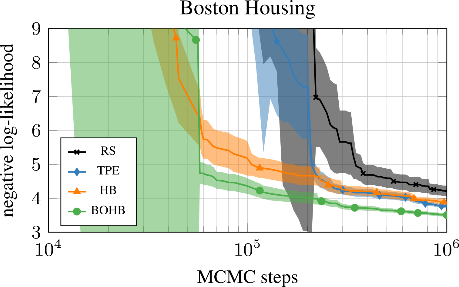
Optimization of 5 hyperparameters of a Bayesian neural network trained with SGHMC on the Boston dataset. Many random hyperparameter configurations lead to negative log-likelihoods orders of magnitude higher than the best performing ones, thus the y-axis is clipped at 9 to ensure visibility in the plot.
Optimization of a reinforcement learning agent
Reinforcement learning is known to be very sensitive to its hyperparameters (Henderson et al., 2017). Using BOHB to optimize the hyperparameters of an agent results in a much more stable agent and demonstrates BOHB’s ability to deal with very noisy optimization problems (desideratum 5). In this experiment, eight hyperparameters of a PPO (Schulman et al., 2017) agent were optimized, which had to learn the cartpole swing-up task.
To find a robust and well-performing configuration, each function evaluation was repeated nine times with different seeds. The average number of episodes until PPO has converged to the optimum is reported. The minimum budget for BOHB and HB was one trial and the maximum budget were nine trials. All other methods used a fixed number of nine trials. The following figure shows that HB and BOBH both worked well in the beginning, but again BOBH converged to better configurations in the end. The budget might not have been sufficient for TPE to find the same well-performing configuration.
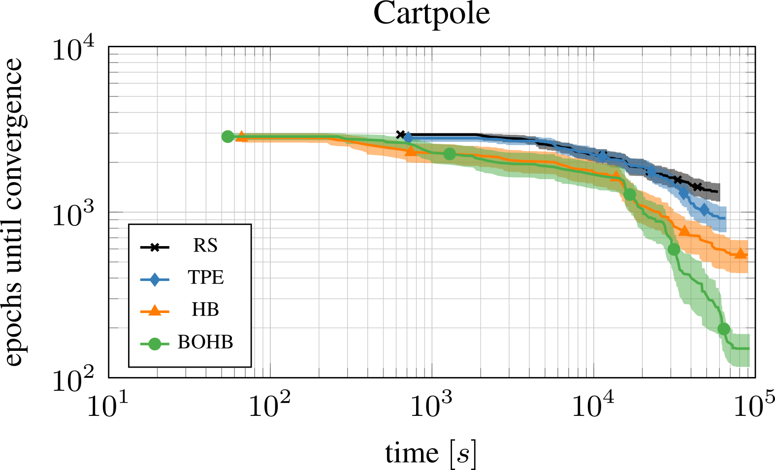
Hyperparameter optimization of 8 hyperparameters of PPO on the cartpole task. BOHB starts as well as HB but converges to a much better configuration.
Optimization of an SVM
BOHB was compared against Gaussian process based BO (GP-BO) with expected improvement, multi-task BO (MTBO; Swersky et al., 2013), Fabolas (Klein et al., 2017) and Random Search (RS) for the optimization of the regularization and the kernel parameter of an SVM on MNIST surrogate (see Klein et al., 2017). The surrogate imitates the optimization of an SVM with an RBF kernel and two hyperparameters. The number of training data points were taken as budget for HB and BOHB, all other methods optimized on the full data set. It is noteworthy that this is a lower-dimensional benchmark on which GP-BO methods usually work better than other methods. Fabolas improved the fastest with Hyperband and BOHB following closely. In fact, Hyperband find the optimal configuration almost always in the first iteration, while BOHB sometimes requires a second iteration. All methods using data subsets converged to the true optimum within 20000 seconds, long before GP-BO and Random Search made any significant progress.
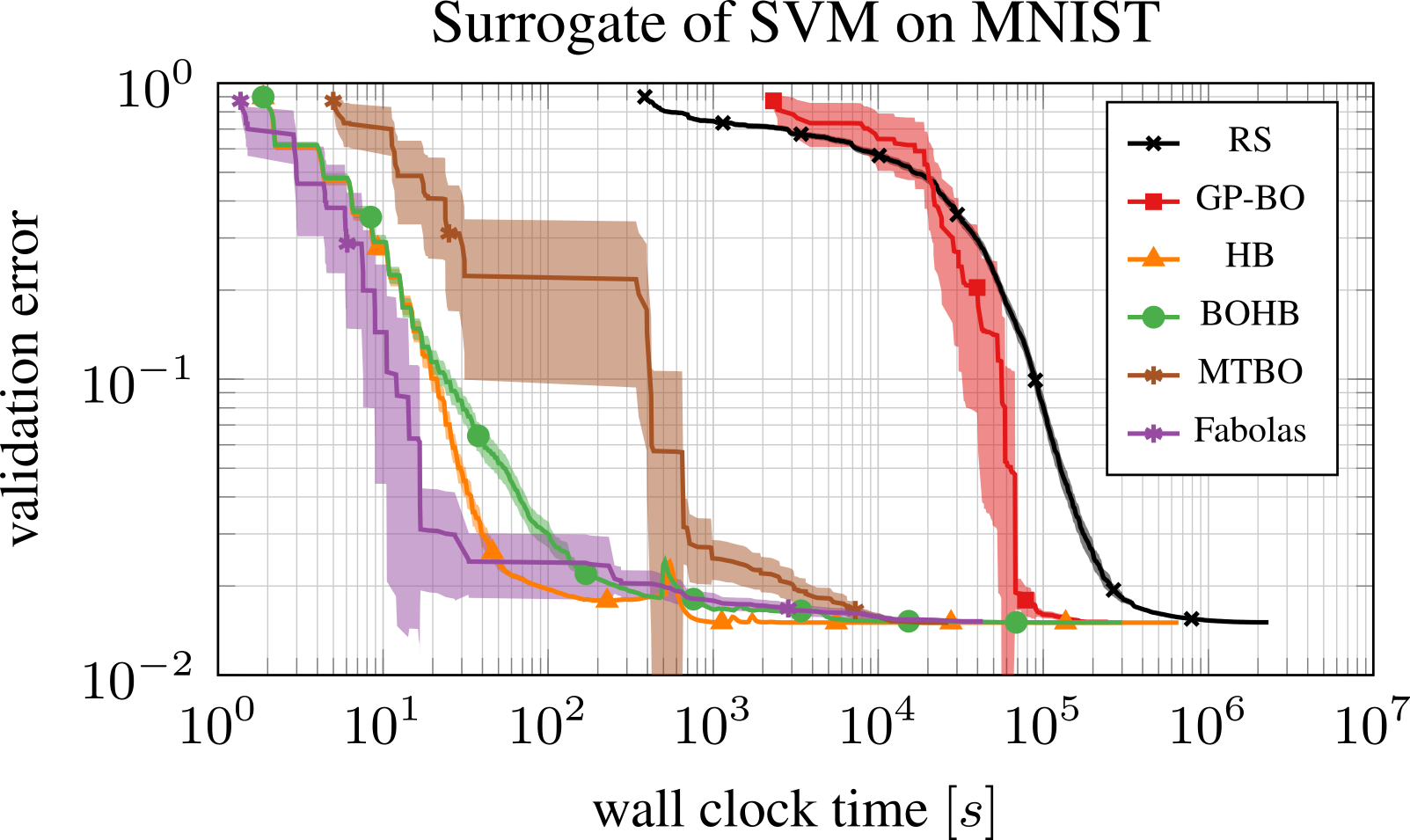
Comparison on the SVM on MNIST surrogates (see Klein et al., 2017). Fabolas outperforms BOHB in the beginning on this two dimensional benchmark, however BOHB outperforms MTBO.
When does BOHB *not* work well?
To use BOHB (and Hyperband), you need to be able to define meaningful budgets: small budgets should yield cheap approximations to your expensive objective function of interest (the full budget), and the relative rankings of different hyperparameter configurations on small budgets should somewhat resemble the relative rankings of those same configurations on the full budget. If evaluations on the small budgets are misleading or just too noisy to really tell you anything about performance with the full budget, then BOHB’s Hyperband component will be wasteful and you’re better off only using the full budget like vanilla Bayesian optimization does. In such cases, you could expect BOHB to be k times slower than standard BO, where k is the number of brackets used in BOHB’s Hyperband component. (This is the same factor that Hyperband may be worse than random search in the worst case.)
Compared to Hyperband, in all examples we have studied, BOHB performed better, but one could construct an adversarial function that “hides” the best hyperparameter configuration in a region of the search space that otherwise yields extremely poor performance. To still converge for such a worst-case response surface, BOHB relies on choosing a fixed fraction (by default 1/3) of the configurations it evaluates uniformly at random (like Hyperband chooses all its configurations). Relying on this strategy, BOHB would be a constant factor (by default: 3 times) slower than Hyperband in the worst case. In practice, we have only ever observed this behaviour on the surprisingly easy SVM experiment, where both methods solved the problem within 2 iteration. Usually, the KDE model usually leads to much faster convergence to the optimum region than random search.
Conclusion
BOHB is a simple yet effective method for hyperparameter optimization satisfying the desiderata outlined above: it is robust, flexible, scalable (to both high dimensions and parallel resources), and achieves both strong anytime performance and strong final performance. The experiments we mentioned demonstrate that BOHB indeed fulfills the given desiderata. But you shouldn’t just blindly trust a blog post, and we thus encourage you to try the implementation of BOHB for yourself (and if you like it use it for your own HPO problems). We’d love to hear your feedback. Examples of how to use BOHB are listed under https://github.com/automl/HpBandSter/tree/master/hpbandster/examples.