In supervised learning, multiple works have investigated training networks using artificial data. For instance, in dataset distillation, the information of a larger dataset is distilled into a smaller synthetic dataset in order to improve train time.
Synthetic environments (SEs) aim to apply a similar idea to Reinforcement learning (RL). They are proxies for real environments that generate artificial state dynamics and rewards which allow faster and more stable training of RL agents. Additionally, this approach can be used to perform Hyperparameter optimization or Neural Architecture search for RL agents more efficiently.
Problem Statement
A Markov Decision Process (MDP) is a 4-Tuple $latex (S,A,P,R)$, with $latex S$ a set of states, $latex A$ a set of action. $latex P : S \times A \rightarrow S$ are the state transition probabilities. Lastly, $latex R$ represents the immediate reward.
In the following, we distinguish between two types of MDPs, human designed environments $latex \mathcal{E}_{real}$ and synthetic learned environments $latex \mathcal{E}_{syn, \psi}$ which are referred to as SEs. SEs are represented by neural networks with parameter $latex \psi$. Given an action $latex a \in A$ and the current state $latex s \in S$, it outputs the next state $latex s’$ and the immediate reward $latex r$. Formally we want to find parameters $latex \psi^*$ such that an agent trained on $latex \mathcal{E}_{syn,\psi^*}$ maximizes the performance on $latex \mathcal{E}_{real}$.
$latex \begin{aligned}
\psi^* &= \underset{\psi}{\text{arg max}} \ F(\theta^*(\psi); \mathcal{E}_{real}) \\
\text{s.t. }\ \theta^*(\psi) &= \underset{\theta}{\text{arg max}}\ F(\theta, \mathcal{E}_{syn, \psi})
\end{aligned}$
Training Synthetic Environments
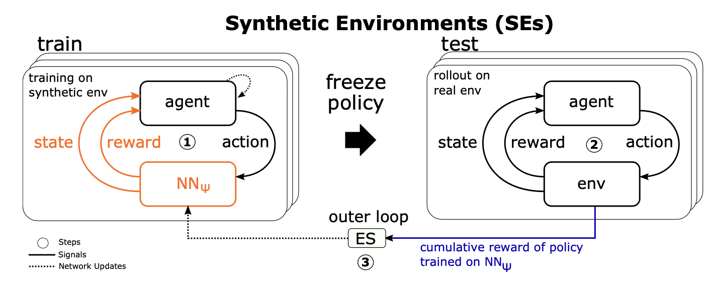
Figure 1: Overview of bi-level optimization scheme for synthetic environments.
The method for training SEs relies on a bi-level optimization scheme, consisting of an inner and outer-loop. The inner-loop trains the RL agent on the SE. As the method is agnostic to both the domain and agent, any standard RL algorithm can be adopted. While the outer loop serves to optimize the SE parameters psi based solely on the cumulative rewards achieved on the real environment. The outer loop optimization is performed using Evolution Strategies with a population of SE parameters.
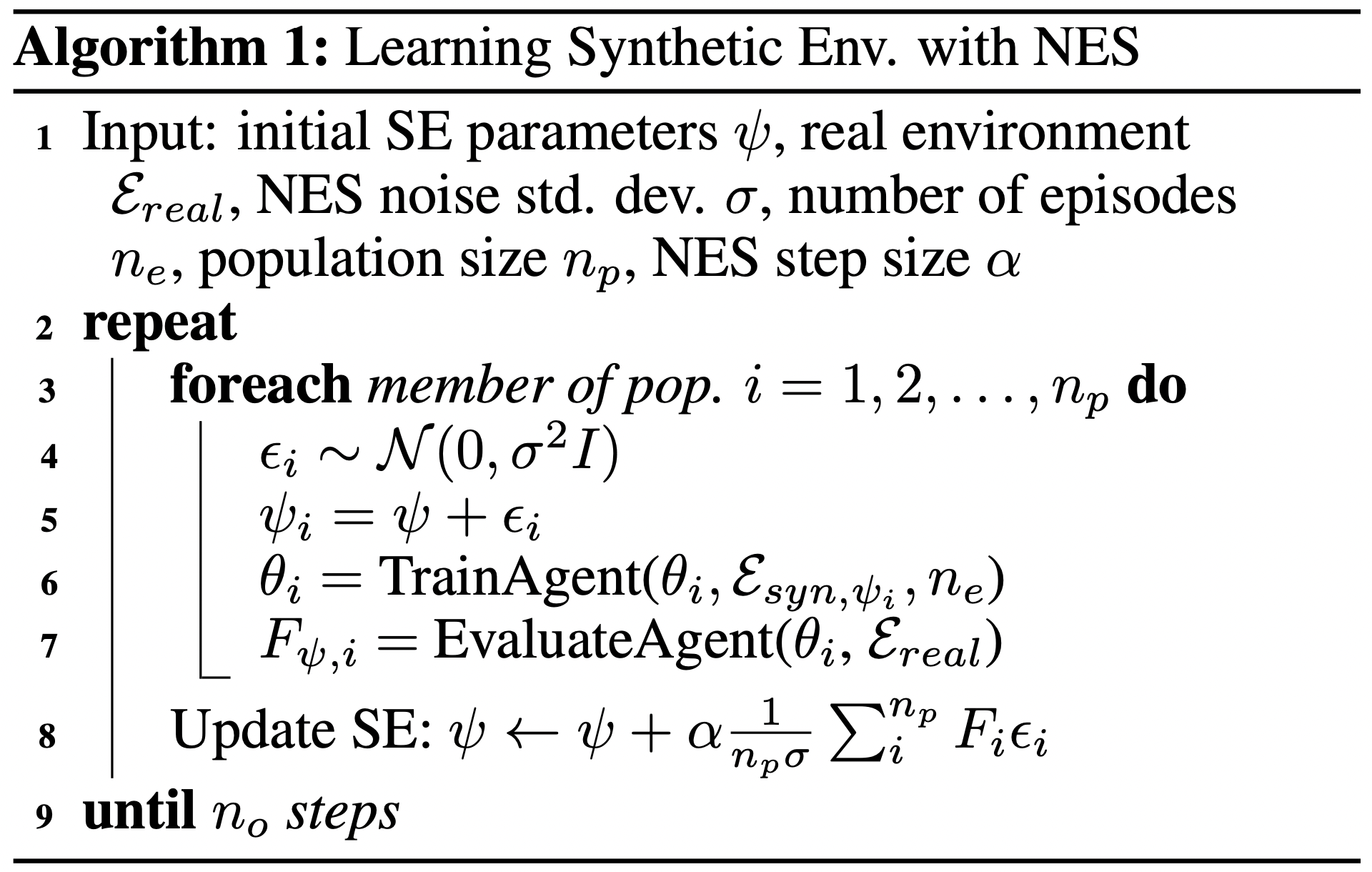
The training of the synthetic environment is depicted in Algorithm 1. First, the SE parameters are initialized, along with the population. For each member of the population, Gaussian noise is added to the SE parameters. Then an agent is trained on the SE $latex \psi_i$ and evaluated on the real environment. The cumulative reward is used as a score. Finally, the parameters are updated using a gradient estimate based on the scores.
Experimental Setup
The experiments are performed on two Gym tasks, CartPole-v0 and Acrobat-v1. For training the SEs we always used DDQN as RL agent. In order to test the transferability of the SEs, robustness to different HPs and training of different agents was tested. Due to known sensitivity to hyperparameters, some of the agents and NES hyperparameters were optimized using BOHB.
Feasibility
Assuming the goal is to identify SEs that allow fast agent training, we may ask first: “Are we able to learn synthetic environments efficiently?”. After identifying stable hyperparameters, SE training was run for 200 outer loop iterations, using 16 workers. Given enough resources, SEs that can train agents on CartPole and Acrobat can be identified. Notably, after 50 NES outer loop steps are often sufficient to solve the real task, as seen in the figure 2.
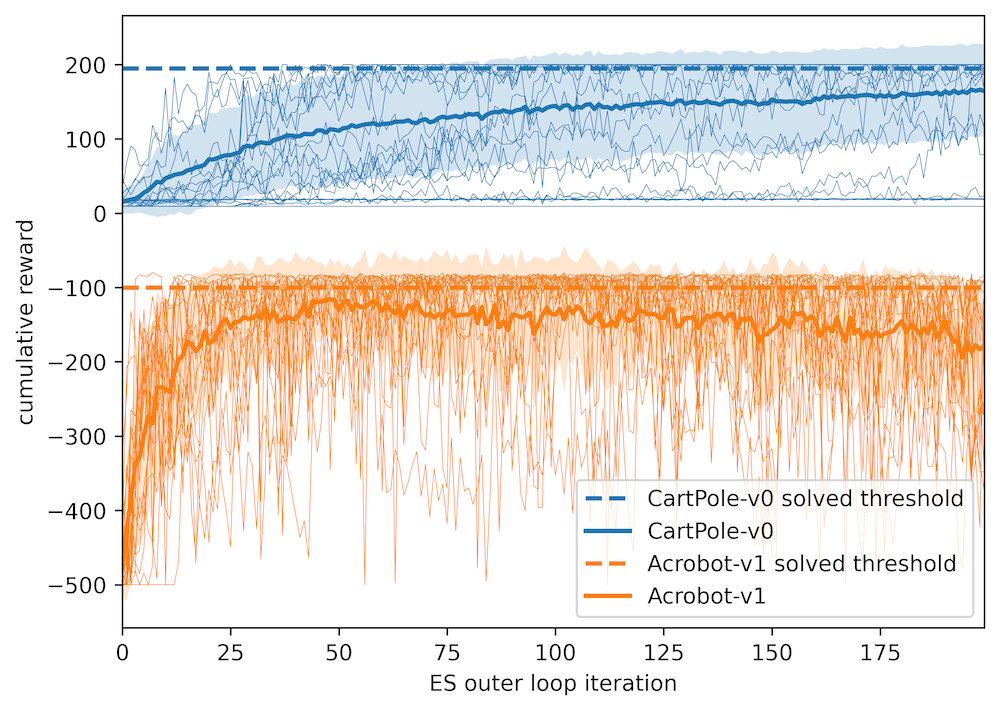
Figure 2: Multiple NES runs for CartPole (top) and Acrobot (bottom). Each thin line corresponds to the average of 16 worker evaluation scores.
Performance
To investigate whether the method can learn SEs, capable of effectively and efficiently training agents, two sets of SEs were trained. For one set, the agent’s HPs were randomly sampled for each inner loop, while for the other set, the HPs were kept constant.
40 synthetic environments were trained for each set, then 10 DDQN agents with randomly sampled HPs were trained on the final SEs, and finally tested for 10 episodes on the real environment. For the baseline, 40 instantiations of the real environment were used which resulted in 4000 evaluations in total for each setting.
Training the SE with fixed HP leads to the worst result, overfitting the SE to the agent’s hyperparameters. When varying the HP during training, SEs are consistently training agents using around 60% fewer steps during training, seen in the bottom left of figure 3. This is achieved while being more stable and less sensitive to the agent’s hyperparameters, as depicted by the densities in figure 3 (top left).
Figure 3: The top row shows the density for the corresponding settings. The bottom row depicts the Average train steps and episodes along with the mean reward (below bars).
Transferability
As the training of SE already requires numerous environment observations, it is difficult to justify the argument of speed improvement. For this reason, transferability of DDQN trained SEs to other agents was tested. Thus, the trained SE from the previous experiments were reused.
First, we start by training a Dueling DDQN with varying HPs. Here, transfer succeeded, again yielding more stable training and a speed-up of around 50% for the SE trained with varying hyperparameters (figure 3 top and bottom center). Again, keeping the HP fixed during SE training negatively impacted the agent’s performance.
To test the performance for an agent outside the deep q-learning class, transferability to TD-3 adapted to handle discrete spaces was explored. While for the baseline (training on real env) the TD-3 is able to solve the environment, training on the SE shows limited transferability (figure 3 top and bottom right). Some SEs are still able to train TD-3 agents and in this case they maintain the efficiency.
Limitations
While SEs yield multiple advantages, they also have some drawbacks. NES strongly depends on the number of workers, requiring a lot of parallel computational resources. This limit was encountered in preliminary experiments with more complex tasks, where 16 workers were not sufficient to learn SEs being capable of learning the tasks. Lastly, Markovian fully observable states were assumed.
SE behavior
After we have seen the advantages and disadvantages of using synthetic environments, can we shed some light on the efficacy of the learned SEs?
As we operate on tasks with small state spaces, we can perform a qualitative visual study, approximately depicting state and reward distribution, in order to get an insight to the inner workings of SEs.
For both the CartPole and Acrobat task, one SE was randomly chosen, and on each SE 10 DDQN agents were trained. During the training all $latex (s,a,r,s’)$ tuples were logged. The SE-trained agents were then evaluated on the real environment for 10 test episodes each, again logging all $latex (s,a,r,s’)$ tuples. Lastly, the occurrence of the next states and rewards are visualized in histograms, color coded according to their origin.
All histograms show a distribution shift between SE and real environment, showing strong performance on barely seen states during training. Furthermore, some synthetic state distributions are narrower than their real counterparts, introducing a bias towards relevant states. Notably, for the rewards, the distribution is wider, indicating sparse rewards becoming dense.
The green histogram depicts the SE response when fed with state-action pairs that the agents have seen during testing. For most states, the green distribution aligns better with the blue one, indicating that SE may guide agents towards relevant states.
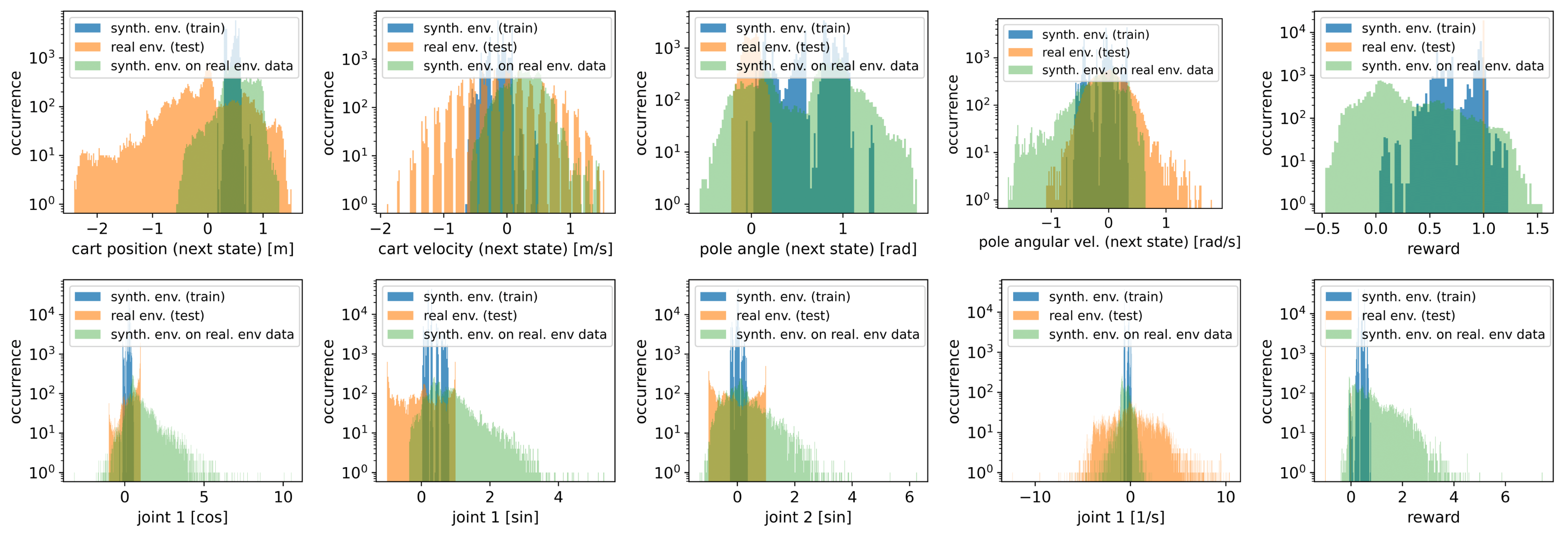
Figure 4: The top row shows the histogram for the next state $latex s’$ and reward $latex r$ produce by 10 DDQN agents trained on a CartPole SE (blue) and afterwards tested for 10 episodes on a real environment (orange). Additionally the SE responses when fed with real data during testing are shown in green. The bottom row shows the same for Acrobot.
More Details!
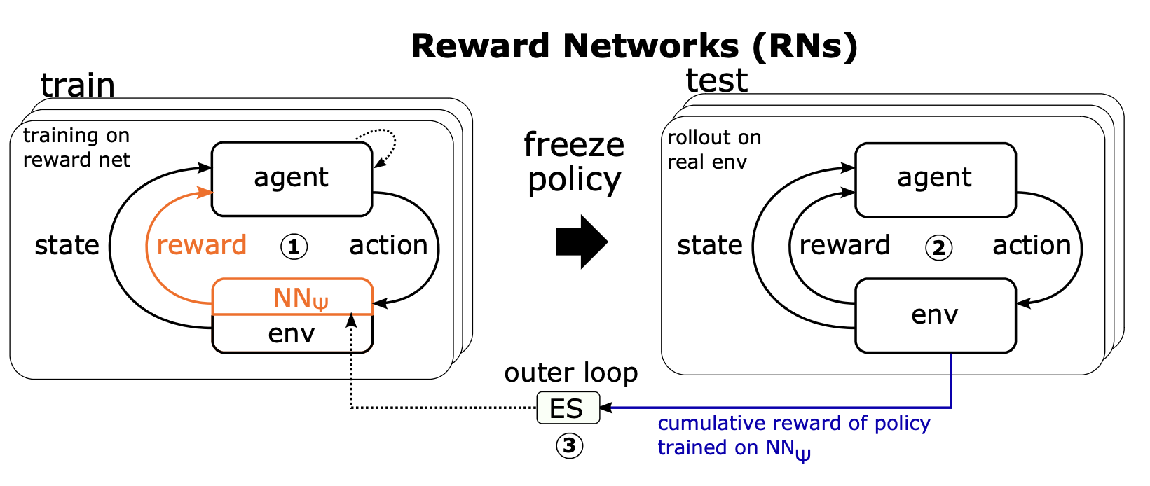
Figure 5: Overview of bi-level optimization scheme for reward networks.
Are you excited to learn more?
We have additional experiments investigating learning reward networks. Reward networks use the same bi-level optimization scheme learning (to augment) rewards, reducing computational complexity while still achieving efficient training.
All details can be found in our ICLR 2022 paper at: https://arxiv.org/abs/2101.09721.
The accompanying code can be found at https://github.com/automl/learning_environments.